Tutorials
Logging
To see logs, use the logging API. The logs can be
useful for keeping track of what is happening behind
the scenes.
import logging
logging.basicConfig()
logging.getLogger().setLevel('INFO')
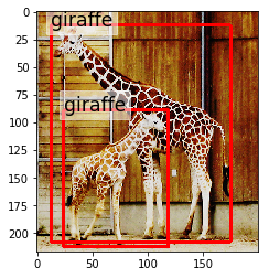
Browsing image data
from mira import datasets
coco = datasets.load_coco2017(subset='val')
coco[26].show()
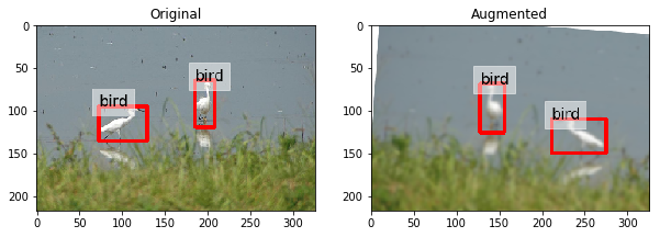
Augmentation
Augmentation can be kind of a pain for
object detection sometimes. But albumentations
makes it pretty easy to build augmentation pipelines
and mira uses a protocol to specify how the augmentation
should work. Note that, if you use albumentations, you
must use the ‘pascal_voc’ format. Alternatively, you can use
an arbitrary function that adheres to the mira.core.utils.AugmenterProtocol
protocol.
from mira import datasets
from mira import core
import albumentations as A

dataset = datasets.load_voc2012(subset='val')
scene = dataset[15]

augmenter = core.augmentations.compose([A.HorizontalFlip(p=1), A.GaussianBlur()])

fig, (ax_original, ax_augmenter) = plt.subplots(ncols=2, figsize=(10, 5))
ax_original.set_title('Original')
ax_augmenter.set_title('Augmented')

scene.show(ax=ax_original)
scene.augment(augmenter)[0].show(ax=ax_augmenter)
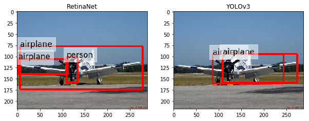
Basic object detection
The example below shows how easy it is to do object detection using the common API for detectors.
from mira import datasets, detectors
import matplotlib.pyplot as plt

# Load the VOC dataset (use the validation
# split to save time)
dataset = datasets.load_voc2012(subset='val')

# Load FasterRCNN with pretrained layers. It is
# set up to use COCO labels.
detector_faster = detectors.FasterRCNN(pretrained_top=True)

detector_retina = detectors.RetinaNet(pretrained_top=True)

# Pick an example scene
scene = dataset[5]

# Set up side-by-side plots
fig, (ax_retinanet, ax_faster) = plt.subplots(ncols=2, figsize=(10, 5))
ax_retinanet.set_title('EfficientDet')
ax_faster.set_title('FasterRCNN')

# We get predicted scenes from each detector. Detectors return
# lists of annotations for a given image. So we can just replace
# (assign) those new annotations to the scene to get a new scene
# reflecting the detector's prediction.
predicted_retinanet = scene.assign(
    annotations=detector_retina.detect(scene.image),
    categories=detector_retina.categories
)
predicted_faster = scene.assign(
    annotations=detector_faster.detect(scene.image, threshold=0.4),
    categories=detector_faster.categories
)

# Plot both predictions. The calls to annotation() get us
# an image with the bounding boxes drawn.
_ = predicted_retinanet.show(ax=ax_retinanet)
_ = predicted_faster.show(ax=ax_faster)
Transfer Learning
This example inspired by the TensorFlow object detection tutorial.
import albumentations as A
from mira import datasets, detectors, core

# Load the Oxford pets datasets with a class
# for each breed.
dataset = datasets.load_oxfordiiitpets(breed=True)

# Load FasterRCNN with pretrained backbone. We'll
# use the annotation configuration for our
# new task.
detector = detectors.FasterRCNN(
    pretrained_top=False,
    pretrained_backbone=True,
    categories=dataset.categories,
)

# Split our dataset into training, validation,
# and test.
trainval, testing = dataset.train_test_split(
    train_size=0.7, test_size=0.3
)
training, validation = trainval.train_test_split(
    train_size=0.66, test_size=0.33
)

# Create an augmenter
augmenter = core.augmentations.compose([A.HorizontalFlip(p=1), A.GaussianBlur()])

# Run training job
detector.train(
    training=training,
    validation=validation,
    epochs=1000,
    batch_size=8,
    augmenter=augmenter,
)
Training on COCO 2014
Start by downloading all of the COCO images. If you haven’t already, install gsutil, which will make downloading the images a snap.
curl https://sdk.cloud.google.com | bash
mkdir coco
cd coco
mkdir images
gsutil -m rsync gs://images.cocodataset.org/train2014 images
gsutil -m rsync gs://images.cocodataset.org/val2014 images
gsutil -m rsync gs://images.cocodataset.org/test2014 images
Now download the annotations. The following will create an annotations folder inside of your coco folder.
curl -LO  http://images.cocodataset.org/annotations/annotations_trainval2014.zip -o annotations_trainval2014.zip
unzip annotations_trainval2014.zip
Let’s load the dataset.
from mira import datasets

training = datasets.load_coco(
    annotations_file='coco/annotations/instances_train2014.json',
    image_dir='coco/images'
)
validation = datasets.load_coco(
    annotations_file='coco/annotations/instances_val2014.json',
    image_dir='coco/images'
)
And now we can train a detector.
from mira import detectors

detector = detectors.FasterRCNN(
    categories=training.categories
)
detector.train(
    training=training,
    validation=validation,
    epochs=1000
)
Deployment
You can deploy your models using TorchServe. The example below exports pretrained models to the MAR format.
import mira.detectors as md

detector1 = md.FasterRCNN(pretrained_top=True, backbone="resnet50")
detector1.to_torchserve("fastrcnn")
detector2 = md.RetinaNet(pretrained_top=True)
detector2.to_torchserve("retinanet")
The above will generate fastrcnn.mar and retinanet.amr in the model-store directory. You can then use those models with TorchServe using:
torchserve --start --model-store model-store --models retinanet=retinanet.mar,fastrcnn=fastrcnn.mar
Then you can do inference in TorchServe using something like the following.
# Get responses from server.
with open("path/to/image.jpg", "rb") as f:
    data = f.read()
    prediction1 = requests.post("http://localhost:8080/predictions/fastrcnn", data=data).json()
    prediction2 = requests.post("http://localhost:8080/predictions/retinanet", data=data).json()
    categories = mc.Categories(list(set(p["label"] for p in prediction1 + prediction2)))
scene1, scene2 = [
    mc.Scene(
        image=filename,
        categories=categories,
        annotations=[
            mc.Annotation(
                x1=p["x1"],
                y1=p["y1"],
                x2=p["x2"],
                y2=p["y2"],
                category=categories[p["label"]],
                score=p["score"]
            ) for p in prediction
        ]
    ) for prediction in [prediction1, prediction2]
]
You can stop the server using torchserve --stop. Note that to restart the server, you should delete the logs directory that torchserve creates as it stores cached state that you may not want.